The Steps of Fuzzy DEMATEL Method
Step 1: Generate the fuzzy direct- relation matrix
In order to identify the model of the relations among the n criteria, an n × n matrix is first generated. The influence of the element in each row exerted on the element in each column of this matrix can be represented a fuzzy number. If multiple experts' opinions are used, all experts must complete the matrix. arithmetic mean of all of the experts' opinions is used to generate the direct relation matrix z.
The table below indicates the direct relation matrix, which is the same as pairwise comparison matrix of the experts.
The direct relation matrix
| A | B | C | D | |
| A | (0.000,0.000,0.000) | (0.000,0.000,0.250) | (0.000,0.000,0.250) | (0.000,0.250,0.500) |
| B | (0.000,0.000,0.250) | (0.000,0.000,0.000) | (0.000,0.000,0.250) | (0.250,0.500,0.750) |
| C | (0.000,0.000,0.250) | (0.000,0.250,0.500) | (0.000,0.000,0.000) | (0.500,0.750,1.000) |
| D | (0.000,0.000,0.250) | (0.000,0.250,0.500) | (0.250,0.500,0.750) | (0.000,0.000,0.000) |
The following table shows the fuzzy scale used in the model.
Fuzzy Scale
| Code | Linguistic terms | L | M | U |
| 1 | No influence | 0 | 0 | 0.25 |
| 2 | Very low influence | 0 | 0.25 | 0.5 |
| 3 | Low influence | 0.25 | 0.5 | 0.75 |
| 4 | High influence | 0.5 | 0.75 | 1 |
| 5 | Very high influence | 0.75 | 1 | 1 |
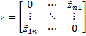
Step 2: Normalize the fuzzy direct-relation matrix
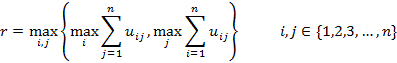
The normalized fuzzy direct-relation matrix can be obtained using the following formula:
![]()
where
The normalized fuzzy direct-relation matrix
| A | B | C | D | |
| A | (0.000,0.000,0.000) | (0.000,0.000,0.111) | (0.000,0.000,0.111) | (0.000,0.111,0.222) |
| B | (0.000,0.000,0.111) | (0.000,0.000,0.000) | (0.000,0.000,0.111) | (0.111,0.222,0.333) |
| C | (0.000,0.000,0.111) | (0.000,0.111,0.222) | (0.000,0.000,0.000) | (0.222,0.333,0.444) |
| D | (0.000,0.000,0.111) | (0.000,0.111,0.222) | (0.111,0.222,0.333) | (0.000,0.000,0.000) |
Step 3: Calculate the fuzzy total-relation matrix
In step 3, the fuzzy total-relation matrix can be calculated by the following formula:
![]()
If each element of the fuzzy total-relation matrix is expressed as
![]() , it can be calculated as follows:
, it can be calculated as follows:
![]()
![]()
![]()
In other words, the normalized matrix the inverse is first calculated, and then it is subtracted from the matrix I, and finally the normalized matrix is multiplied by the resulting matrix. The following table shows the fuzzy direct-relation matrix.
The fuzzy total-relation matrix
| A | B | C | D | |
| A | (0.000,0.000,0.126) | (0.000,0.017,0.308) | (0.000,0.028,0.325) | (0.000,0.124,0.497) |
| B | (0.000,0.000,0.254) | (0.000,0.034,0.257) | (0.013,0.055,0.383) | (0.114,0.248,0.646) |
| C | (0.000,0.000,0.308) | (0.000,0.165,0.532) | (0.025,0.089,0.379) | (0.228,0.400,0.859) |
| D | (0.000,0.000,0.284) | (0.000,0.152,0.491) | (0.114,0.248,0.581) | (0.025,0.116,0.485) |
Step 4: Defuzzify into crisp values
The CFCS method proposed by Opricovic and Tzeng has been used to obtain a crisp value of total-relation matrix. The steps of CFCS method are as follows:
![]()
![]()
![]()
So that
![]()
Calculating the upper and lower bounds of normalized values:
![]()
![]()
The output of the CFCS algorithm is crisp values.
Calculating total normalized crisp values:
![]()
The crisp total-relation matrix
| A | B | C | D | |
| A | 0.02 | 0.067 | 0.079 | 0.184 |
| B | 0.043 | 0.071 | 0.113 | 0.307 |
| C | 0.051 | 0.209 | 0.138 | 0.45 |
| D | 0.048 | 0.194 | 0.284 | 0.178 |
Step 5: set the threshold value
The threshold value must be obtained in order to calculate the internal relations matrix. Accordingly, partial relations are neglected and the network relationship map (NRM) is plotted. Only relations whose values in matrix T is greater than the threshold value are depicted in the NRM. To compute the threshold value for relations, it is sufficient to calculate the average values of the matrix T. After the threshold intensity is determined, all values in matrix T which are smaller than the threshold value are set to zero, that is, the causal relation mentioned above is not considered.
In this study, the threshold value is equal to 0.152
All the values in matrix T which are smaller than 0.152 are set to zero, that is, the causal relation mentioned above is not considered. The model of significant relations is presented in the following table.
The crisp total- relationships matrix by considering the threshold value
| A | B | C | D | |
| A | 0 | 0 | 0 | 0.184 |
| B | 0 | 0 | 0 | 0.307 |
| C | 0 | 0.209 | 0 | 0.45 |
| D | 0 | 0.194 | 0.284 | 0.178 |
Step 6: Final output and create a causal relation diagram
The next step is to find out the sum of each row and each column of T (in step 4). The sum of rows (D) and columns (R) can be calculated as follows:
![]()
![]()
Then, the values of D+R and D-R can be calculated by D and R, where D+R represent the degree of importance of factor i in the entire system and D-R represent net effects that factor i contributes to the system.
The table below shows the final output.
The final output
| R | D | D+R | D-R | |
| A | 0.163 | 0.35 | 0.512 | 0.187 |
| B | 0.541 | 0.534 | 1.075 | -0.007 |
| C | 0.614 | 0.848 | 1.462 | 0.234 |
| D | 1.118 | 0.704 | 1.823 | -0.414 |
The following figure shows the model of significant relations. This model can be represented as a diagram in which the values of (D+R) are placed on the horizontal axis and the values of (D-R) on the vertical axis. The position and interaction of each factor with a point in the coordinates (D+ R, D-R) are determined by coordinate system.
cause-effect diagram
Step 7: Interpret the results
According to the diagram and table above, each factor can be assessed based on the following aspects:
- Horizontal vector (D + R) represents the degree of importance between each factor plays in the entire system. In other words, (D + R) indicates both factor i’s impact on the whole system and other system factors’ impact on the factor. in terms of degree of importance, D is ranked in first place and C, B and A, are ranked in the next places.
- The vertical vector (D-R) represents the degree of a factor’s influence on system. In general, the positive value of D-R represents a causal variable, and the negative value of D-R represents an effect. In this study, A, C are considered to be as a causal variable, B, D are regarded as an effect.