 Download Word
 Download Excel
 Print
Print
TOPSIS as one of MCDM methods considers both the distance of each alternative from the positive ideal and the distance of each alternative from the negative ideal point. In other words, the best alternative should have the shortest distance from the positive ideal solution (PIS) and the longest distance from the negative ideal.
In this study there are 4 criteria and 5 alternatives that are ranked based on TOPSIS method. The following table describes the criteria
Characteristics of Criteria
| name | type | weight | |
| 1 | Throughput capacity | Positive | 0.3 |
| 2 | Integration flexibility | Positive | 0.25 |
| 3 | Annual operating cost | Negative | 0.25 |
| 4 | Implementation lead time | Positive | 0.2 |
The following table shows the decision matrix.
Decision Matrix
| Throughput capacity | Integration flexibility | Annual operating cost | Implementation lead time | |
| Dematic AGV System | 5 | 4 | 3 | 2 |
| Swisslog AutoStore | 4 | 5 | 2 | 3 |
| Geek+ RoboShuttle | 3 | 4 | 1 | 4 |
| Honeywell Intelligrated | 4 | 3 | 2 | 5 |
| Vanderlande ADAPTO | 5 | 4 | 2 | 3 |
The Steps of the TOPSIS Method :
STEP 1: Normalize the decision-matrix.
The following formula can be used to normalize.

The following table shows the normalized matrix.
The normalized matrix
| Throughput capacity | Integration flexibility | Annual operating cost | Implementation lead time | |
| Dematic AGV System | 0.524 | 0.442 | 0.64 | 0.252 |
| Swisslog AutoStore | 0.419 | 0.552 | 0.426 | 0.378 |
| Geek+ RoboShuttle | 0.314 | 0.442 | 0.213 | 0.504 |
| Honeywell Intelligrated | 0.419 | 0.331 | 0.426 | 0.63 |
| Vanderlande ADAPTO | 0.524 | 0.442 | 0.426 | 0.378 |
STEP 2: Calculate the weighted normalized decision matrix.
According to the following formula, the normalized matrix is multiplied by the weight of the criteria.

The following table shows the weighted normalized decision matrix.
The weighted normalized matrix
| Throughput capacity | Integration flexibility | Annual operating cost | Implementation lead time | |
| Dematic AGV System | 0.157 | 0.11 | 0.16 | 0.05 |
| Swisslog AutoStore | 0.126 | 0.138 | 0.107 | 0.076 |
| Geek+ RoboShuttle | 0.094 | 0.11 | 0.053 | 0.101 |
| Honeywell Intelligrated | 0.126 | 0.083 | 0.107 | 0.126 |
| Vanderlande ADAPTO | 0.157 | 0.11 | 0.107 | 0.076 |
STEP 3: Determine the positive ideal and negative ideal solutions.
The aim of the TOPSIS method is to calculate the degree of distance of each alternative from positive and negative ideals. Therefore, in this step, the positive and negative ideal solutions are determined according to the following formulas.


So that


where j1 and j2 denote the negative and positive criteria, respectively.
The following table shows both positive and negative ideal values.
The positive and negative ideal values
| Positive ideal | Negative ideal | |
| Throughput capacity | 0.157 | 0.094 |
| Integration flexibility | 0.138 | 0.083 |
| Annual operating cost | 0.053 | 0.16 |
| Implementation lead time | 0.126 | 0.05 |
STEP4: distance from the positive and negative ideal solutions
TOPSIS method ranks each alternative based on the relative closeness degree to the positive ideal and distance from the negative ideal. Therefore, in this step, the calculation of the distances between each alternative and the positive and negative ideal solutions is obtained by using the following formulas.

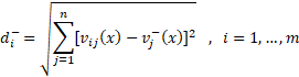
The following table shows the distance to the positive and negative ideal solutions.
Distance to positive and negative ideal points
| Distance to positive ideal | Distance to positive negative | |
| Dematic AGV System | 0.134 | 0.069 |
| Swisslog AutoStore | 0.08 | 0.087 |
| Geek+ RoboShuttle | 0.073 | 0.121 |
| Honeywell Intelligrated | 0.083 | 0.098 |
| Vanderlande ADAPTO | 0.078 | 0.091 |
STEP 5: Calculate the relative closeness degree of alternatives to the ideal solution
In this step, the relative closeness degree of each alternative to the ideal solution is obtained by the following formula. If the relative closeness degree has value near to 1, it means that the alternative has shorter distance from the positive ideal solution and longer distance from the negative ideal solution.
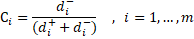
The following table shows the relative closeness degree of each alternative to the ideal solution and its ranking.
The ci value and ranking
| Ci | rank | |
| Dematic AGV System | 0.34 | 5 |
| Swisslog AutoStore | 0.521 | 4 |
| Geek+ RoboShuttle | 0.623 | 1 |
| Honeywell Intelligrated | 0.541 | 2 |
| Vanderlande ADAPTO | 0.536 | 3 |
The following figure shows the ci values.
The ci value